PhD Update: July 2016

The majority of July has been focused on widening the applications of the Area class in PyTrx, which is being developed to determine real world areal data from oblique photography. Specifically I have been working on detecting visible plume extent. Unlike surface lake extent, plume detection has proved difficult to automate due to poor contrast. However, I have made an alternative set of functions to manually distinguish plume extent which look promising for yielding high-frequency, high-resolution areal data.

A submarine plume is an upwelling of freshwater from an ocean-terminating glacier terminus. A sediment-rich, 'muddy' area of water forms in cases where this upwelling reaches the ocean surface. This upwelling is largely caused by the density difference between fresh water and salt water, creating a column of turbulent water that promotes melting of the glacier front in its immediate vicinity. This submarine melting is considered to be one of the main controls on ice calving in tidewater settings. Plumes also provide significant feeding grounds for birds, seals and other local wildlife in the area - small organisms (which survive in saltwater) are stunned when they come into contact with freshwater from the glacier and are transported to the surface via the upwelling plume column. Birds feed off these stunned organisms at the surface whilst seals and other sea life feed from organisms entrained in the upwelling plume column.

A submarine plume emerging at the ocean surface in front of Tunabreen glacier in Svalbard (August 2015)

Monitoring the areal extent of plumes is thus vital to understanding current and future glacier dynamics and wildlife feeding tendencies. Building on the automated detection of surface lakes (for more information, click here), I first attempted to automate the detection of plume extent from oblique time-lapse images based on pixel intensity (i.e. the RBG signature that denotes the 'colour' of a pixel). Unlike the detection of lakes, the contrast between the plume and surrounding fjord water is often quite poor. Sunlight glare off the water surface can also create false extents and obscure the plume (see example in the GIF sequence below).

A sample of our time-lapse images from Kronebreen glacier, Svalbard. This sequence covers twelve hours (real-time) from 9am-9pm during the peak summer melt season, with one image taken every hour. A submarine plume can be seen in the foreground growing and shrinking through the course of the day.

In most instances the plume extent needed to be manually defined, hence I created a collection of functions within PyTrx* for manual extent definition. The extent is defined by manually plotting points onto the image that denote the plume's boundary. The first GIF below shows those points plotted on to each image, forming polygons that show the plume's extent over a twelve hour period (9am - 9pm, July 2015).  The plume extent grows and subsides over the course of a day during the summer melt season.

These points are projected from the image plane to the real-world scene using a process called georectification, for which the following parameters need to be known:

1. Camera location
2. Camera pose (represented as the camera's yaw, pitch and roll)
3. Discrepancies between the image plane and the real-world scene created by assymetry in the camera lens and misalignment between the camera lens and camera sensor (called the radial and tangential distortions)
4. Known geographical points in the landscape, such as peaks and geographical features
5. Digitial Elevation Model (DEM) of the landscape.

These parameters are used to mathematically represent the translation between the image environment and the real-world environment. The real world coordinates of the points can then be used to calculate the actual area of the plume extent, simply by forming polygons from the set of coordinates.

Plume detection in the image scene and projection to the real-world environment (polygon overlaid onto a scene from Landsat). Note: the projection is slightly wrong as you can see the plume origin is slightly off-centre from the ice embayment. We are still trying to diagnose why this is happening. It is likely to be an unknown anomaly in the projection, or a mismatch between the polygon and Landsat datums.

This short twelve-hour sequence shows promising results and the method will next be implemented on larger image sequences to observe longer-term variations in plume extent. It is expected that the plume extent is controlled by melt volume, the rate at which melt is transferred to the glacier front, fjord temperature/salinity and prevailing wind direction. Over the twelve hour period studied here, it is likely that the plume extent is controlled by changes in melt volume, which is understood to increase and decrease on a daily basis. There are few longer-term observations of plume dynamics at such a high temporal resolution, so it will be interesting to see exactly how a plume evolves over a summer melt season.

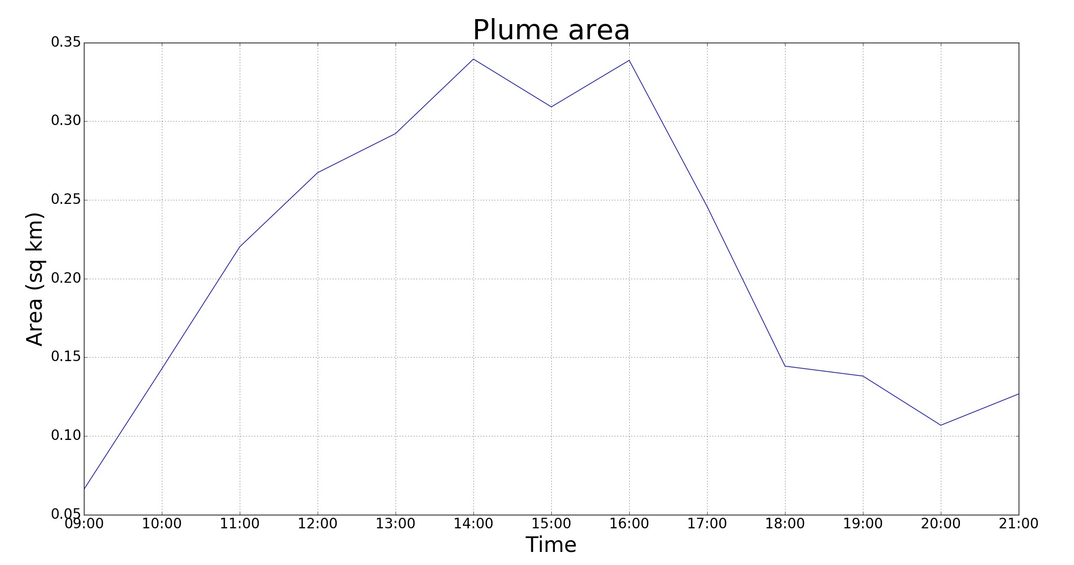
Graph showing plume extent over the course of a twelve-hour period in the summer melt season at Kronebreen glacier, Svalbard. These areas have been calculated using PyTrx and the set of functions for manual extent detection and projection.

---

* PyTrx is a set of photogrammetry tools specifically designed to obtain measurements (length, area and velocity) from oblique photography in glacial environments. PyTrx is programmed in Python and largely uses functions from the OpenCV toolbox. The first version of PyTrx will be made freely available at some point in the near future.